!pip3 install networkx matplotlib python-louvain community13 Network Data
Abstract.
Many types of data, especially social media data, can often be represented as networks. This chapter introduces igraph (R and Python) and networkx (Python) to showcase how to deal with such data, perform Social Network Analysis (SNA), and represent it visually.
Keywords. graphs, social network analysis
Objectives:
- Understand how can networks be represented and visualized
- Conduct basic description of networks
- Perform Social Network Analysis
13.1 Representing and Visualizing Networks
How can networks help us to understand and represent social problems? How can we use social media as a source for small and large-scale network analysis? In the computational analysis of communication these questions become highly relevant given the huge amount of social media data produced every minute on the Internet. In fact, although graph theory and SNA were already being used during the last two decades of the 20th century, we can say that the widespread adoption of the Internet and especially social networking services such as Twitter and Facebook really unleashed their potential. Firstly, computers made it easier to compute graph measures and visualize their general and communal structures. Secondly, the emergence of a big spectrum of social media network sites (i.e. Facebook, Twitter, Sina Weibo, Instagram, Linkedin, etc.) produced an unprecedented number of online social interactions, which still is certainly an excellent arena to apply this framework. Thus, the use of social media as a source for network analysis has become one of the most exciting and promising areas in the field of computational social science.
This section presents a brief overview of graph structures (nodes and edges) and types (directed, weighted, etc.), together with their representations in R and Python. We also include visual representations and basic graph analysis.
A graph is a structure derived from a set of elements and their relationships. The element could be a neuron, a person, an organization, a street, or even a message, and the relationship could be a synapse, a trip, a commercial agreement, a drive connection or a content transmission. This is a different way to represent, model and analyze the world: instead of having rows and columns as in a typical data frame, in a graph we have nodes (components) and edges (relations). The mathematical representation of a graph \(G=(V,E)\) is based on a set of nodes (also called vertices): \(\{v_{1}, v_{2},\ldots v_{n}\}\) and the edges or pair of nodes: \(\{(v_{1}, v_{2}), (v_{1}, v_{3}), (v_{2},v_{3}) \ldots (v_{m}, v_{n}) \in E\}\) As you may imagine, it is a very versatile procedure to represent many kinds of situations that include social, media, or political interactions. In fact, if we go back to 1934 we can see how graph theory (originally established in the 18th century) was first applied to the representation of social interactions (Moreno 1934) in order to measure the attraction and repulsion of individuals of a social group1.
The network approach in social sciences has an enormous potential to model and predict social actions. There is empirical evidence that we can successfully apply this framework to explain distinct phenomena such as political opinions, obesity, and happiness, given the influence of our friends (or even of the friends of our friends) over our behavior (Christakis and Fowler 2009). The network created by this sophisticated structure of human and social connections is an ideal scenario to understand how close we are to each other in terms of degrees of separation (Watts 2004) in small (e.g., a school) and large-scale (e.g., a global pandemic) social dynamics. Moreover, the network approach can help us to track the propagation either of a virus in epidemiology, or a fake news story in political and social sciences, such as in the work by Vosoughi, Roy, and Aral (2018).
Now, let us show you how to create and visualize network structures in R and Python. As we mentioned above, the structure of a graph is based on nodes and edges, which are the fundamental components of any network. Suppose that we want to model the social network of five American politicians in 2017 (Donald Trump, Bernie Sanders, Hillary Clinton, Barack Obama and John McCain), based on their imaginary connections on Facebook (friending) and Twitter (following)2. Technically, the base of any graph is a list of edges (written as pair of nodes that indicate the relationships) and a list of nodes (some nodes might be isolated without any connection!). For instance, the friendship on Facebook between two politicians would normally be expressed as two strings separated by comma (e.g., “Hillary Clinton”, “Donald Trump”). In Example 13.1 we use libraries igraph (R)3 and networkx (Python) to create from scratch a simple graph with five nodes and five edges, using the above-mentioned structure of pairs of nodes (notice that we only include the edges while the vertices are automatically generated).
In both cases we generated a graph object g1 which contains the structure of the network and different attributes (such as number_of_nodes() in networkx). You can add/remove nodes and edges to/from this initial graph, or even modify the names of the vertices. One of the most useful functions is the visualization of the network (plot in igraph and draw or draw_networkx in networkx). Example 13.2 shows a basic visualization of the imaginary network of friendships of five American politicians on Facebook.
Example 13.2 Visualization of a simple graph.
nx.draw_networkx(g1)

pos = nx.shell_layout(g1)
x_values, y_values = zip(*pos.values())
x_max = max(x_values)
x_min = min(x_values)
x_margin = (x_max - x_min) * 0.40
plt.xlim(x_min - x_margin, x_max + x_margin)plt.box(False)
plt.show()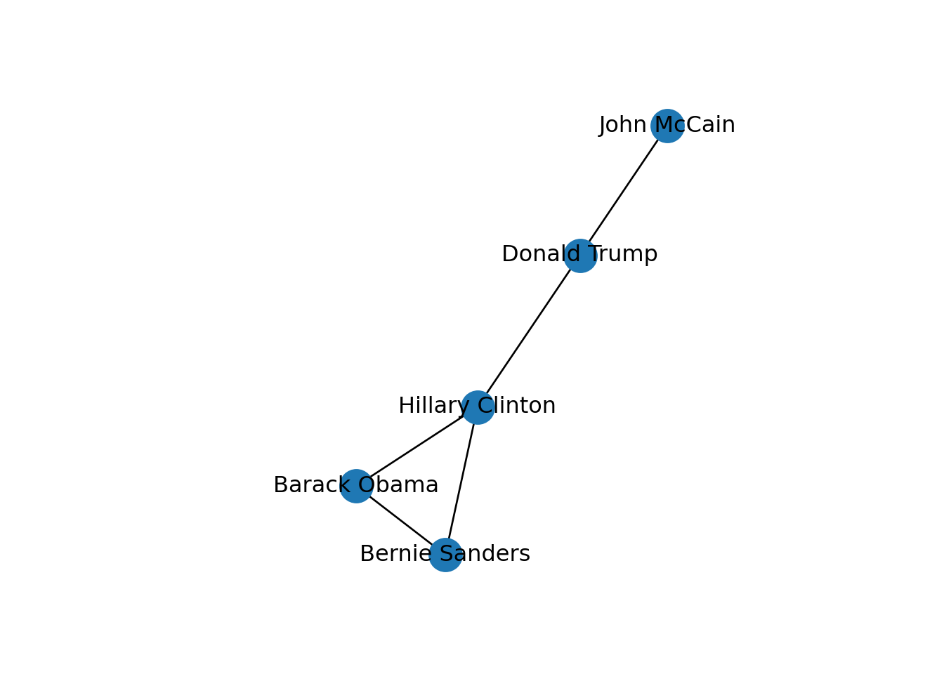
plot(g1)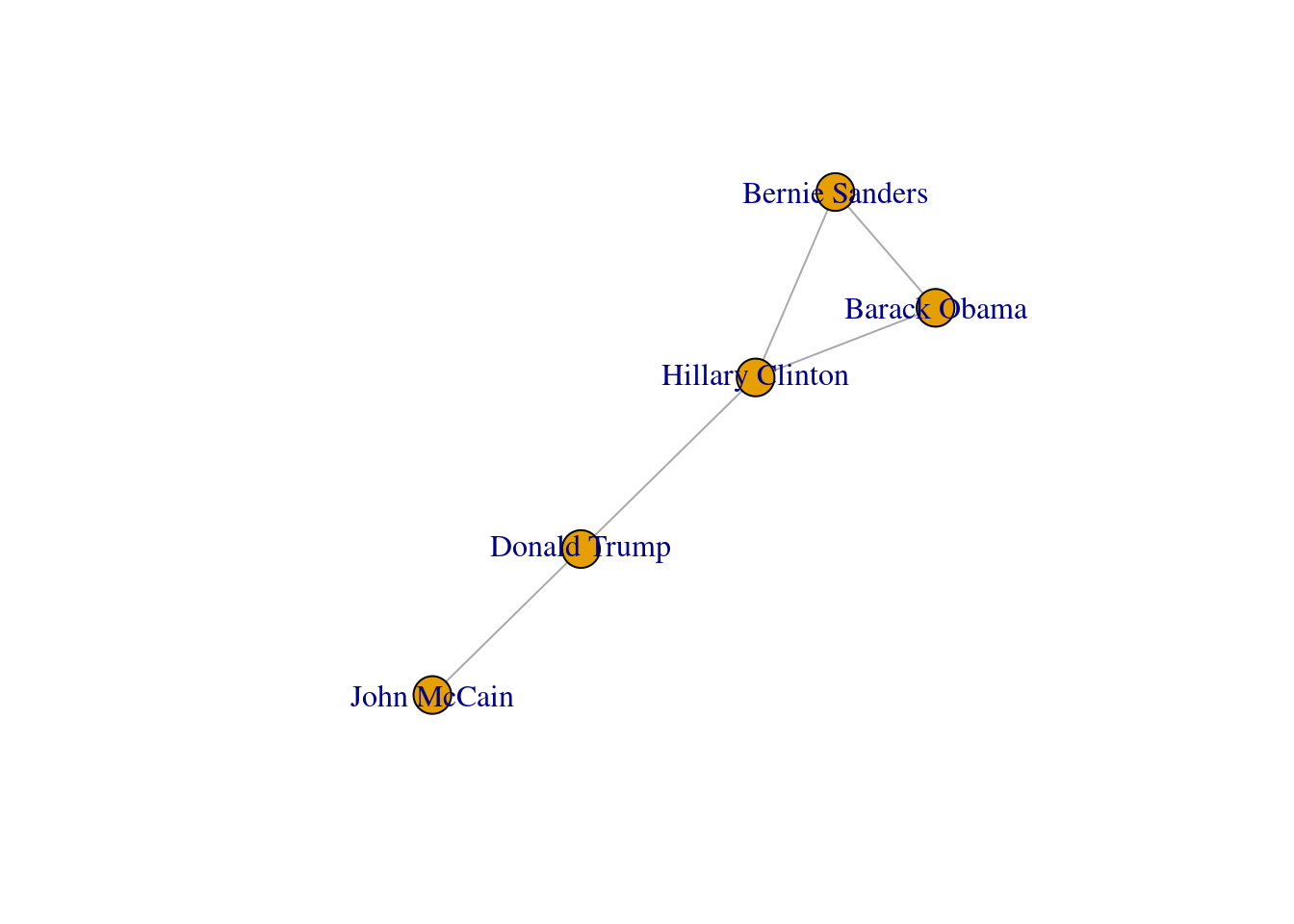
Using network terminology, either nodes or edges can be adjacent or not. In the figure we can say that nodes representing Donald Trump and John McCain are adjacent because they are connected by an edge that depicts their friendship. Moreover, the edges representing the friendships between John McCain and Donald Trump, and Hillary Clinton and Donald Trump, are also adjacent because they share one node (Donald Trump).
Now that you know the relevant terminology and basics of working with graphs, you might be wondering: what if I want to do the same with Twitter? Can I represent the relationships between users in the very same way as Facebook? Well, when you model networks it is extremely important that you have a clear definition of what you mean with nodes and edges, in order to maintain a coherent interpretation of the graph. In both, Facebook and Twitter, the nodes represent the users, but the edges might not be the same. In Facebook, an edge represents the friendship between two users and this link has no direction (once a user accepts a friend request, both users become friends). In the case of Twitter, an edge could represent various relationships. For example, it could mean that two users follow each other, or that one user is following another user, but not the other way around! In the latter case, the edge has a direction, which you can establish in the graph. When you give directions to the edges you are creating a directed graph. In Example 13.3 the directions are declared with the order of the pair of nodes: the first position is for the “from” and the second for the “to”. In igraph (R) we set the argument directed of the function make_graph to TRUE. In networkx (Python), you use the class DiGraph instead of Graph to create the object g2.
In the new graph the edges represent the action of following a user on Twitter. The first declared edge indicates that Hillary Clinton follows Donald Trump, but does not indicate the opposite. In order to provide the directed graph with more arrows we included in g2 two new edges (Obama following Clinton and Clinton following Sanders), so we can have a couple of reciprocal relationships besides the unidirectional ones. You can visualize the directed graph in Example 13.4 and see how the edges now contain useful arrows.
Example 13.4 Visualization of a directed graph.
nx.draw_networkx(g2)

pos = nx.shell_layout(g2)
x_values, y_values = zip(*pos.values())
x_max = max(x_values)
x_min = min(x_values)
x_margin = (x_max - x_min) * 0.40
plt.xlim(x_min - x_margin, x_max + x_margin)plt.box(False)
plt.show()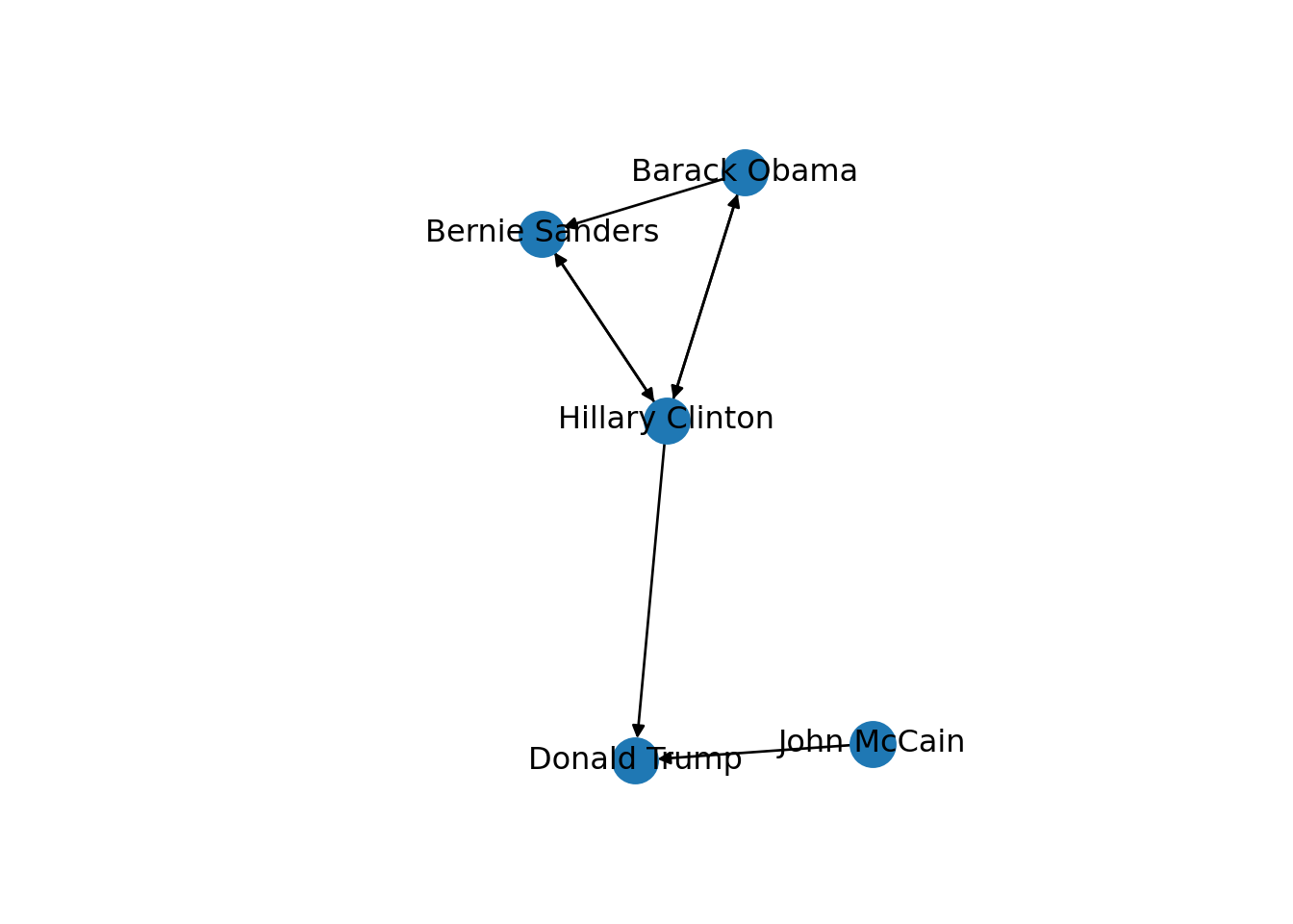
plot(g2)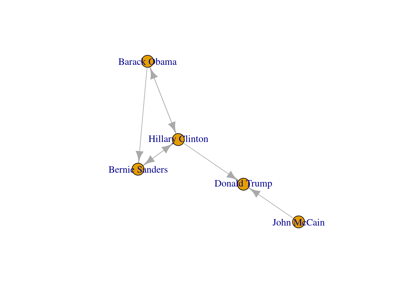
The edges and nodes of our graph can also have weights and features or attributes. When the edges have specific values that depict a feature of every pair of nodes (i.e., the distance between two cities) we say that we have a weighted graph. This type of graph is extremely useful for creating a more accurate representation of a network. For example, in our hypothetical network of American politicians on Twitter (g2) we can assign weights to the edges by including the number of likes that each politician has given to the followed user. This value can serve as a measure of the distance between the nodes (i.e., the higher the number of likes the shorter the social distance). In Example 13.5 we include the weights for each edge: Clinton has given five likes to Trumps’ tweets, Sanders 20 to Clinton’s messages, and so on. In the plot you can see how the sizes of the lines between the nodes change as a function of the weights.
Example 13.5 Visualization of a weighted graph
edges_w = [
    ("Hillary Clinton", "Donald Trump", 5),
    ("Bernie Sanders", "Hillary Clinton", 20),
    ("Hillary Clinton", "Barack Obama", 30),
    ("John McCain", "Donald Trump", 40),
    ("Barack Obama", "Hillary Clinton", 50),
    ("Hillary Clinton", "Bernie Sanders", 10),
    ("Barack Obama", "Bernie Sanders", 15),
]
g2 = nx.DiGraph()
g2.add_weighted_edges_from(edges_w)

edge_labels = dict(
    [
        (
            (
                u,
                v,
            ),
            d["weight"],
        )
        for u, v, d in g2.edges(data=True)
    ]
)

nx.draw_networkx_edge_labels(g2, pos, edge_labels=edge_labels)
nx.draw_networkx(g2, pos)
pos = nx.spring_layout(g2)
x_values, y_values = zip(*pos.values())
x_max = max(x_values)
x_min = min(x_values)
x_margin = (x_max - x_min) * 0.40
plt.xlim(x_min - x_margin, x_max + x_margin)plt.box(False)
plt.show()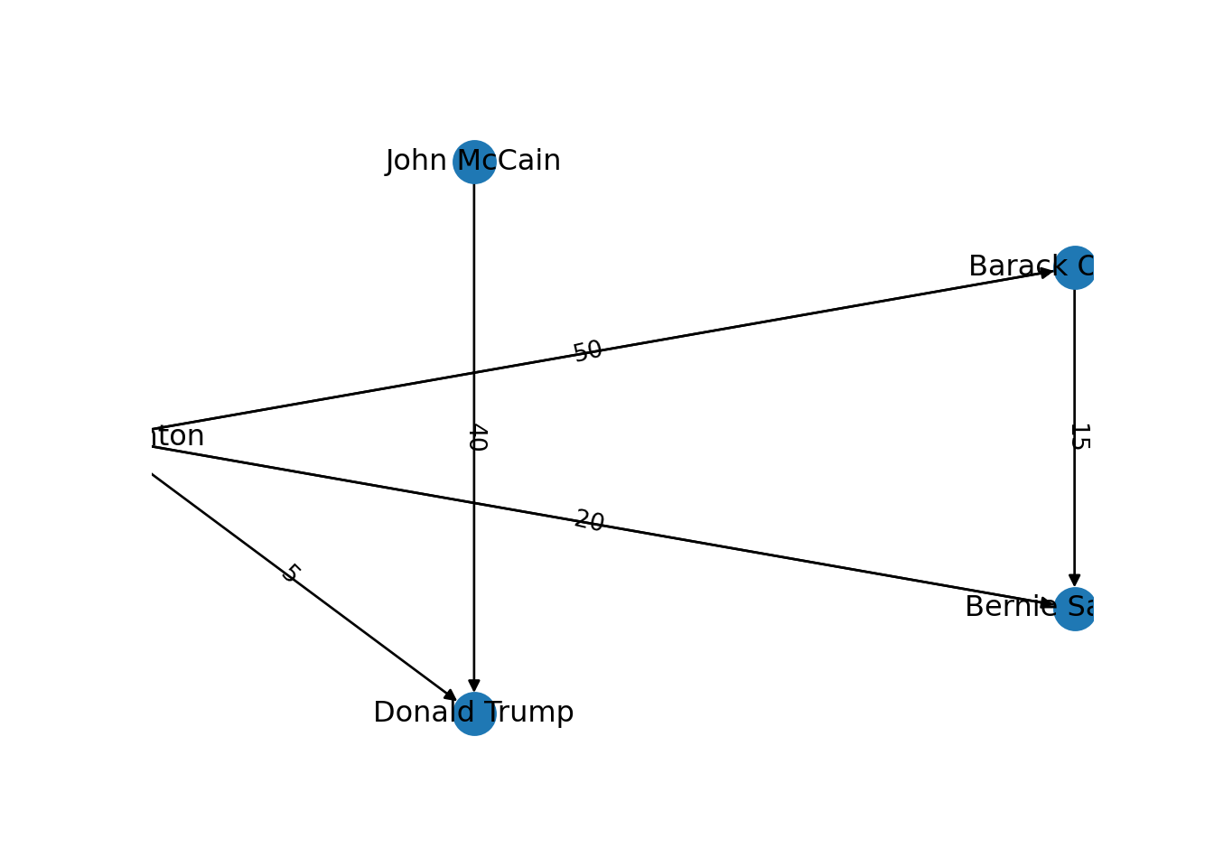
E(g2)$weight = c(5, 20, 30, 40, 50, 10, 15)
plot(g2, edge.label = E(g2)$weight)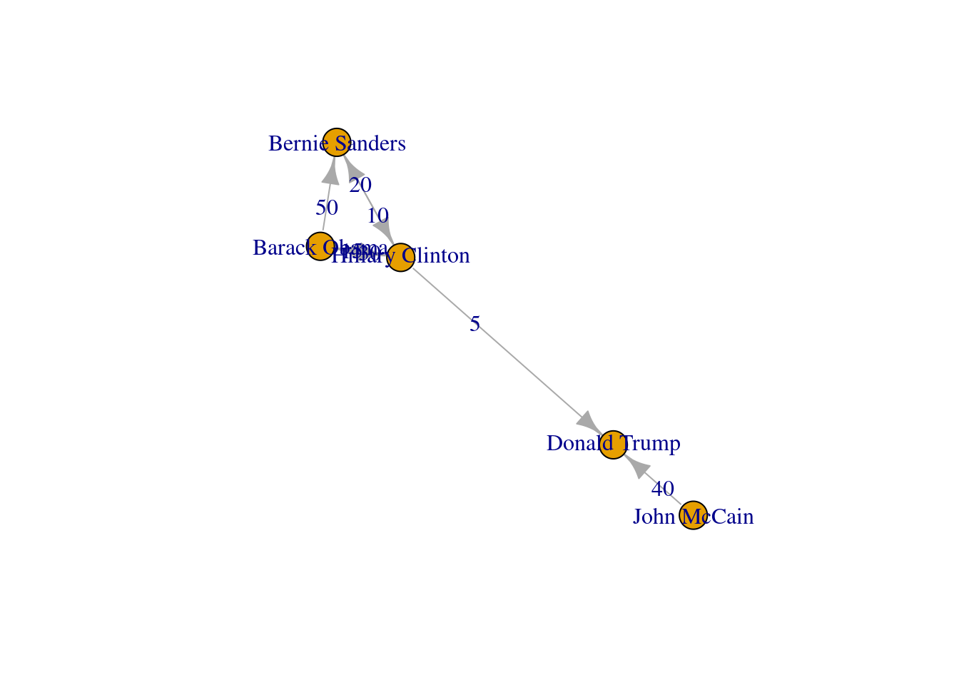
You can include more properties of the components of your graph. Imagine you want to use the number of followers of each politician to determine the size of the nodes, or the gender of the user to establish a color. In Example 13.6 we added the variable followers to each of the nodes and asked the packages to plot the network using this value as the size parameter (in fact we multiplied the values by 0.001 to make it realistic on the screen, but you could also normalize these values when needed). We also included the variable party that was later recoded in a new one called color in order to represent Republicans with red and Democrats with blue. You may need to add other features to the nodes or edges, but with this example you have an overview of what you can do.
Example 13.6 Visualization of a weighted graph including vertex sizes.
attrs = {
    "Hillary Clinton": {"followers": 100000, "party": "Democrat"},
    "Donald Trump": {"followers": 200000, "party": "Republican"},
    "Bernie Sanders": {"followers": 50000, "party": "Democrat"},
    "Barack Obama": {"followers": 500000, "party": "Democrat"},
    "John McCain": {"followers": 40000, "party": "Republican"},
}
nx.set_node_attributes(g2, attrs)
size = nx.get_node_attributes(g2, "followers")
size = list(size.values())

colors = nx.get_node_attributes(g2, "party")
colors = list(colors.values())
colors = [w.replace("Democrat", "blue") for w in colors]
colors = [w.replace("Republican", "red") for w in colors]

nx.draw_networkx_edge_labels(g2, pos, edge_labels=edge_labels)
nx.draw_networkx(
g2, pos, node_size=[x * 0.002 for x in size], node_color=colors
)
pos = nx.spring_layout(g2)
x_values, y_values = zip(*pos.values())
x_max = max(x_values)
x_min = min(x_values)
x_margin = (x_max - x_min) * 0.40
plt.xlim(x_min - x_margin, x_max + x_margin)plt.box(False)
plt.show()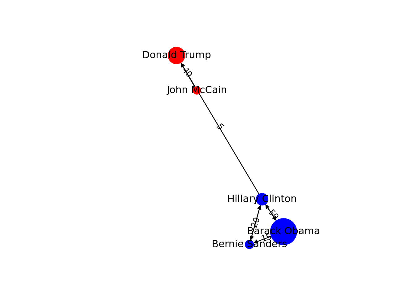
V(g2)$followers = c(100000, 200000,
                    50000,500000, 40000)
V(g2)$party = c("Democrat", "Republican",
            "Democrat", "Democrat", "Republican")
V(g2)$color = V(g2)$party
V(g2)$color = gsub("Democrat", "blue",
                   V(g2)$color)
V(g2)$color = gsub("Republican", "red",
                   V(g2)$color)
plot(g2, edge.label = E(g2)$weight,
     vertex.size = V(g2)$followers*0.0001)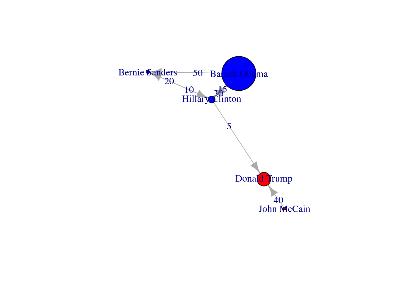
We can mention a third type of graphs: the induced subgraphs, which are in fact subsets of nodes and edges of a bigger graph. We can represent these subsets as \(G' = V', E'\). In Example 13.7 we extract two induced subgraphs from our original network of American politicians on Facebook (g1): the first (g3) is built with the edges that contain only Democrat nodes, and the second (g4) with edges formed by Republican nodes. There is also a special case of an induced subgraph, called a clique, which is an independent or complete subset of an undirected graph (each node of the clique must be connected to the rest of the nodes of the subgraph).
Keep in mind that in network visualization you can always configure the size, shape and color of your nodes or edges. It is out of the scope of this book to go into more technical details, but you can always check the online documentation of the recommended libraries.
So far we have created networks from scratch, but most of the time you will have to create a graph from an existing data file. This means that you will need an input data file with the graph structure, and some functions to load them as objects onto your workspace in R or Python. You can import graph data from different specific formats (e.g., Graph Modeling Language (GML), GraphML, JSON, etc.), but one popular and standardized procedure is to obtain the data from a text file containing a list of edges or a matrix. In Example 13.8 we illustrate how to read graph data in igraph and networkx using a simple adjacency list that corresponds to our original imaginary Twitter network of American politicians (g2).
Example 13.8 Reading a graph from a file
url = "https://cssbook.net/d/poltwit.csv"
fn, _headers = urllib.request.urlretrieve(url)
g2 = nx.read_adjlist(fn, create_using=nx.DiGraph, delimiter=",")
print("Nodes:", g2.number_of_nodes(), "Edges: ", g2.number_of_edges())
Nodes: 5 Edges: 7edges = read_csv(
"https://cssbook.net/d/poltwit.csv",
col_names=FALSE)
g2 = graph_from_data_frame(d=edges)
glue("Nodes: ", gorder(g2),
" Edges: ", gsize(g2))Nodes: 5 Edges: 7plot(g2)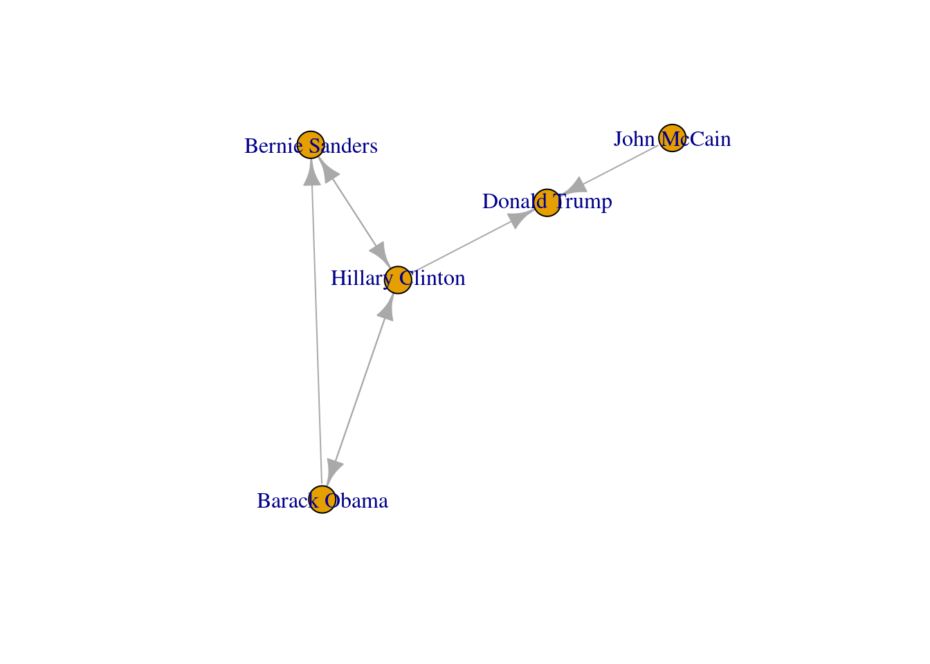
13.2 Social Network Analysis
This section gives an overview of the existing measures to conduct Social Network Analysis (SNA). Among other functions, we explain how to examine paths and reachability, how to calculate centrality measures (degree, closeness, betweenness, eigenvector) to quantify the importance of a node in a graph, and how to detect communities in the graph using clustering.
13.2.1 Paths and Reachability
The first idea that comes to mind when analyzing a graph is to understand how their nodes are connected. When multiple edges create a network we can observe how the vertices constitute one or many paths that can be described. In this sense, a sequence between node x and node y is a path where each node is adjacent to the previous. In the imaginary social network of friendship of American politicians contained in the undirected graph g1, we can determine the sequences or simple paths between any pair of politicians. As shown in Example 13.9 we can use the function all_simple_paths contained in both igraph (R) and networkx (Python), to obtain the two possible routes between Barack Obama and John McCain. The shortest path includes the nodes Hillary Clinton and Donald Trump; and the longer includes Sanders, Clinton, and Trump.
One specific type of path is the one in which the initial node is the same than the final node. This closed path is called a circuit. To understand this concept let us recover the inducted subgraph of Democrat politicians (g3) in which we only have three nodes. If you plot this graph, as we do in Example 13.10, you can clearly visualize how a circuit works.
Example 13.10 Visualization of a circuit.
nx.draw_networkx(g3)
pos = nx.shell_layout(g3)
x_values, y_values = zip(*pos.values())
x_max = max(x_values)
x_min = min(x_values)
x_margin = (x_max - x_min) * 0.40
plt.xlim(x_min - x_margin, x_max + x_margin)plt.box(False)
plt.show()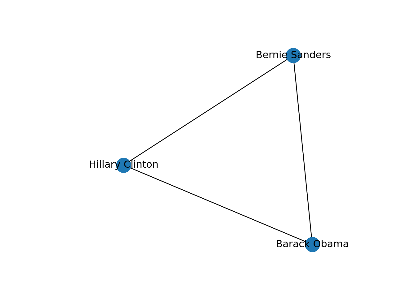
plot(g3)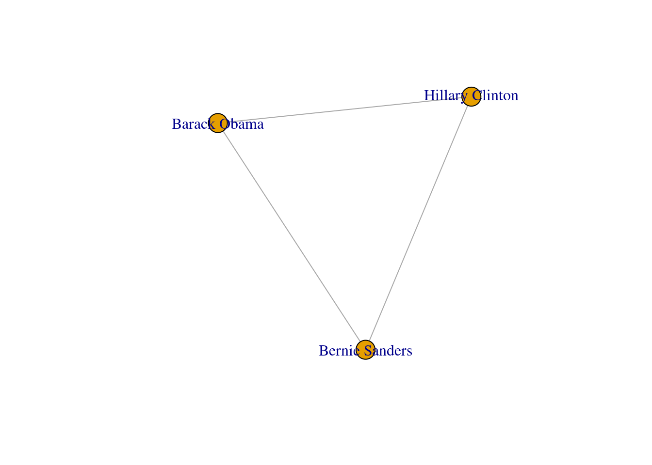
In SNA it is extremely important to be able to describe the possible paths since they help us to estimate the reachability of the vertices. For instance, if we go back to our original graph of American politicians on Facebook (g1) visualized in Example 13.2, we can see that Sanders is reachable from McCain because there is a path between them (McCain–Trump–Clinton–Sanders). Moreover, we observe that this social network is fully connected because you can reach any given node from any other node in the graph. But it might not always be that way. Imagine that we remove the friendship of Clinton and Trump by deleting that specific edge. As you can observe in Example 13.11, when we create and visualize the graph g6 without this edge we can see that the network is no longer fully connected and it has two components. Technically speaking, we would say for example that the subgraph of Republicans is a connected component of the network of American politicians, given that this connected subgraph is part of the bigger graph while not connected to it.
Example 13.11 Visualization of connected components.
# Remove the friendship between Clinton and Trump
g6 = g1.copy()
g6.remove_edge("Hillary Clinton", "Donald Trump")
nx.draw_networkx(g6)
pos = nx.shell_layout(g6)
x_values, y_values = zip(*pos.values())
x_max = max(x_values)
x_min = min(x_values)
x_margin = (x_max - x_min) * 0.40
plt.xlim(x_min - x_margin, x_max + x_margin)plt.box(False)
plt.show()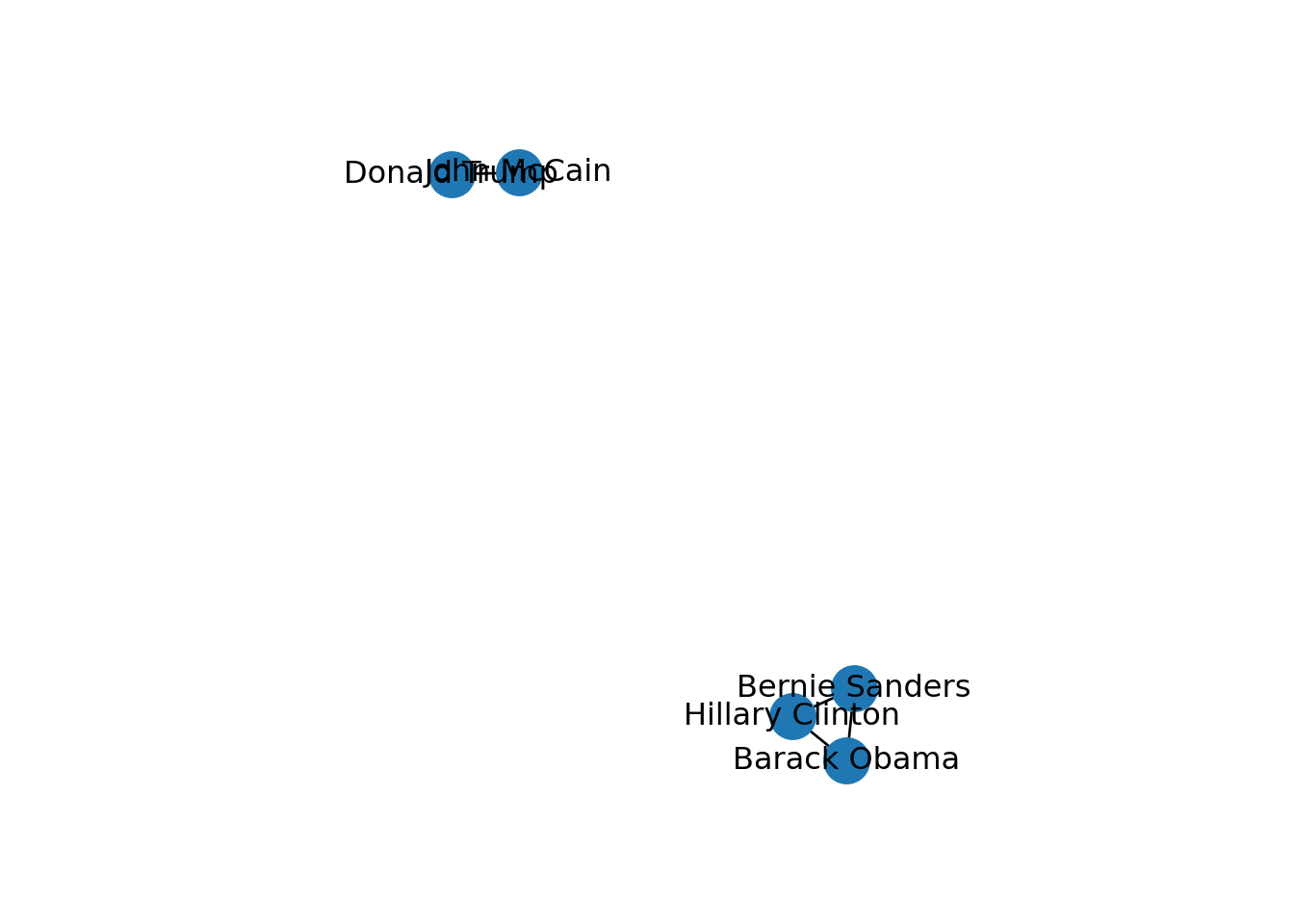
#Remove the friendship between Clinton and Trump
g6 = delete.edges(g1, E(g1, P=
            c("Hillary Clinton","Donald Trump")))
plot(g6)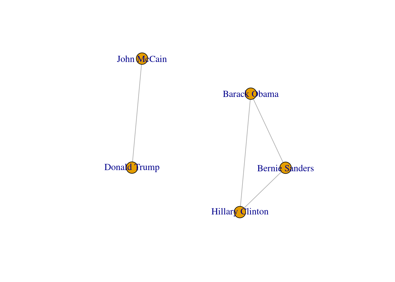
When analyzing paths and reachability you may be interested in knowing the distances in your graph. One common question is what is the average path length of a social network, or in other words, what is the average of the shortest distance between each pair of vertices in the graph? This mean distance can tell you a lot about how close the nodes in the network are: the shorter the distance the closer the nodes are. Moreover, you can estimate the specific distance (shortest path) between two specific nodes. As shown in Example 13.12 we can estimate the average path length (1.7) in our imaginary Facebook network of American politicians using the functions mean_distance in igraph and average_shortest_path_length in networkx. In this example we also estimate the specific distance in the network between Obama and McCain (3) using the function distances in igraph and estimating the length (len) of the shortest path (first result of shortest_simple_paths minus 1) in networkx.
In terms of distance, we can also wonder what the edges or nodes that share a border with any given vertex are. In the first case, we can identify the incident edges that go out or into one vertex. As shown in Example 13.13, by using the functions incident in igraph and edges in networkx we can easily get incident edges of John McCain in the Facebook Network (g1), which is just one single edge that joins Trump with McCain. In the second case, we can also identify its adjacent nodes, or in other words its neighbors. In the very same example, we use neighbors (same function in igraph and networkx) to obtain all the nodes one step away from McCain (in this case only Trump).
There are some other interesting descriptors of social networks. One of the most common measures is the density of the graph, which accounts for the proportion of edges relative to all possible ties in the network. In simpler words, the density tells us from 0 to 1 how much connected the nodes of a graph are. This can be estimated for both undirected and directed graphs. Using the functions edge_density in igraph and density in networkx we obtain a density of 0.5 (middle level) in the imaginary Facebook network of American politicians (undirected graph) and 0.35 in the Twitter network (directed graph).
In undirected graphs we can also measure transitivity (also known as clustering coefficient) and diameter. The first is a key property of social networks that refers to the ratio of triangles over the total amount of connected triples. It is to say that we wonder how likely it is that two nodes are connected if they share a mutual neighbor. Applying the function transitivity (included in igraph and networkx) to g1 we can see that this tendency is of 0.5 in the Facebook network (there is a 50% probability that two politicians are friends when they have a common contact). The second descriptor, the diameter, depicts the length of the network in terms of the longest geodesic distance4. We use the function diameter (included in igraph and networkx) in the Facebook network and get a diameter of 3, which you can also check if you go back to the visualization of g1 in Example 13.2.
Additionally, in directed graphs we can calculate the reciprocity, which is just the proportion of reciprocal ties in a social network and can be computed with the function reciprocity (included in igraph and networkx). For the imaginary Twitter network (directed graph) we get a reciprocity of 0.57 (which is not bad for a Twitter graph where important people usually have much more followers than follows!).
In Example 13.14 we show how to estimate these four measures in R and Python. Notice that in some of the network descriptors you have to decide whether or not to include the edge weights for computation (in the provided examples we did not take these weights into account).
13.2.2 Centrality Measures
Now let us move to centrality measures. Centrality is probably the most common, popular, or known measure in the analysis of social networks because it gives you a clear idea of the importance of any of the nodes within a graph. Using its measures you can pose many questions such as which is the most central person in a network of friends on Facebook, who can be considered an opinion leader on Twitter or who is an influencer on Instagram. Moreover, knowing the specific importance of every node of the network can help us to visualize or label only certain vertices that overpass a previously determined threshold, or to use the color or size to distinguish the most central nodes from the others. There are four typical centrality measures: degree, closeness, eigenvector and betweenness.
The degree of a node refers to the number of ties of that vertex, or in other words, to the number of edges that are incident to that node. This definition is constant for undirected graphs in which the directions of the links are not declared. In the case of directed graphs, you will have three options to measure the degree. First, you can think of the number of edges pointing into a node, which we call indegree; second, we have the number of edges pointing out of a node, or outdegree. In addition, we could also have the total number of edges pointing (in and out) any node. Degree, as well as other measures of centrality mentioned below, can be expressed in absolute numbers, but we can also normalize5 these measures for better interpretation and comparison. We will prefer this latter approach in our examples, which is also the default option in many SNA packages.
We can then estimate the degree of two of our example networks. In Example 13.15, we first estimate the degree of each of the five American politicians in the imaginary Facebook network, which is an undirected graph; and then the total degree in the Twitter network, which is a directed graph. For both cases, we use the functions degree in igraph (R) and degree_centrality in networkx (Python). We later compute the in and out degree for the Twitter network. Using igraph we again used the function degree but now adjust the parameter mode to in or out, respectively. Using networkx, we employ the functions in_degree_centrality and out_degree_centrality.
There are three other types of centrality measures. Closeness centrality refers to the geodesic distance of a node to the rest of nodes in the graph. Specifically, it indicates how close a node is to the others by taking the length of the shortest paths between the vertices. Eigenvector centrality takes into account the importance of the surrounding nodes and computes the centrality of a vertex based on the centrality of its neighbors. In technical words, the measure is proportional to the sum of connection centralities. Finally, betweenness centrality indicates to what extent the node is in the paths that connect many other nodes. Mathematically it is computed as the sum of the fraction of every pair of (shortest) paths that go through the analyzed node.
As shown in Example 13.16, we can obtain these three measures from undirected graphs using the functions closeness, eigen_centrality and betweenness in igraph, and closeness_centrality, eigenvector_centrality and betweenness_centrality in networkx. If we take a look to the centrality measures for every politician of the imaginary Facebook network we see that Clinton seems to be a very important and central node of the graph, just coinciding with the above-mentioned findings based on the degree. It is not a rule that we obtain the very same trend in each of the centrality measures but it is likely that they have similar results although they are looking for different dimensions of the same construct.
We can use these centrality measures in many ways. For example, you can take the degree centrality as a parameter of the node size and labeling when plotting the network. This may be of great utility since the reader can visually identify the most important nodes of the network while minimizing the visual impact of those that are less central. In Example 13.17 we decided to specify the size of the nodes (parameters vertex.size in igraph and node_size in networkx) with the degree centrality of each of the American politicians in the Twitter network (directed graph) contained in g2. We also used the degree centrality to filter the labels in the graph, and then included only those that overpassed a threshold of 0.5 (parameters vertex.label in igraph and labels in networkx). These two simple parameters of the plot give you a fair image of the potential of the centrality measures to describe and understand your social network.
Example 13.17 Using the degree centrality to change the size and labels of the nodes
size = list(nx.degree_centrality(g2).values())
size = [x * 1000 for x in size]
labels_filtered = {k: v for k, v in nx.degree_centrality(g2).items() if v > 0.5}
labels = {}
for k, v in labels_filtered.items():
    labels[k] = k

nx.draw_networkx(g2, node_size=size, labels=labels)

pos = nx.shell_layout(g2)
x_values, y_values = zip(*pos.values())
x_max = max(x_values)
x_min = min(x_values)
x_margin = (x_max - x_min) * 0.40
plt.xlim(x_min - x_margin, x_max + x_margin)plt.box(False)
plt.show()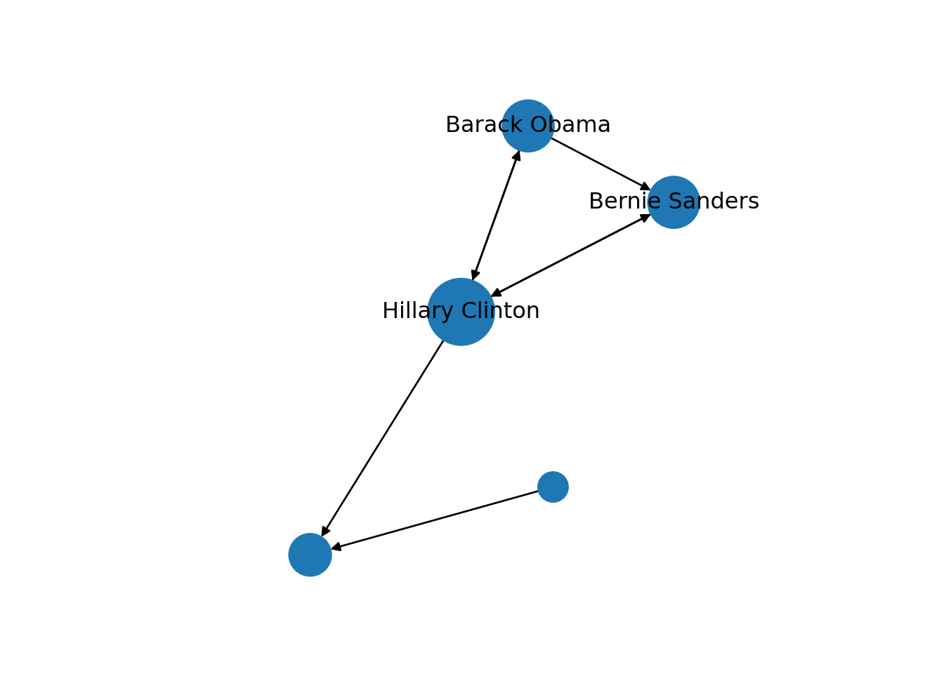
plot(g2, vertex.label.cex = 2,
     vertex.size= degree(g2, normalized = T)*40,
     vertex.label = ifelse(degree(g2,
        normalized = T) > 0.5, V(g2)$name, NA))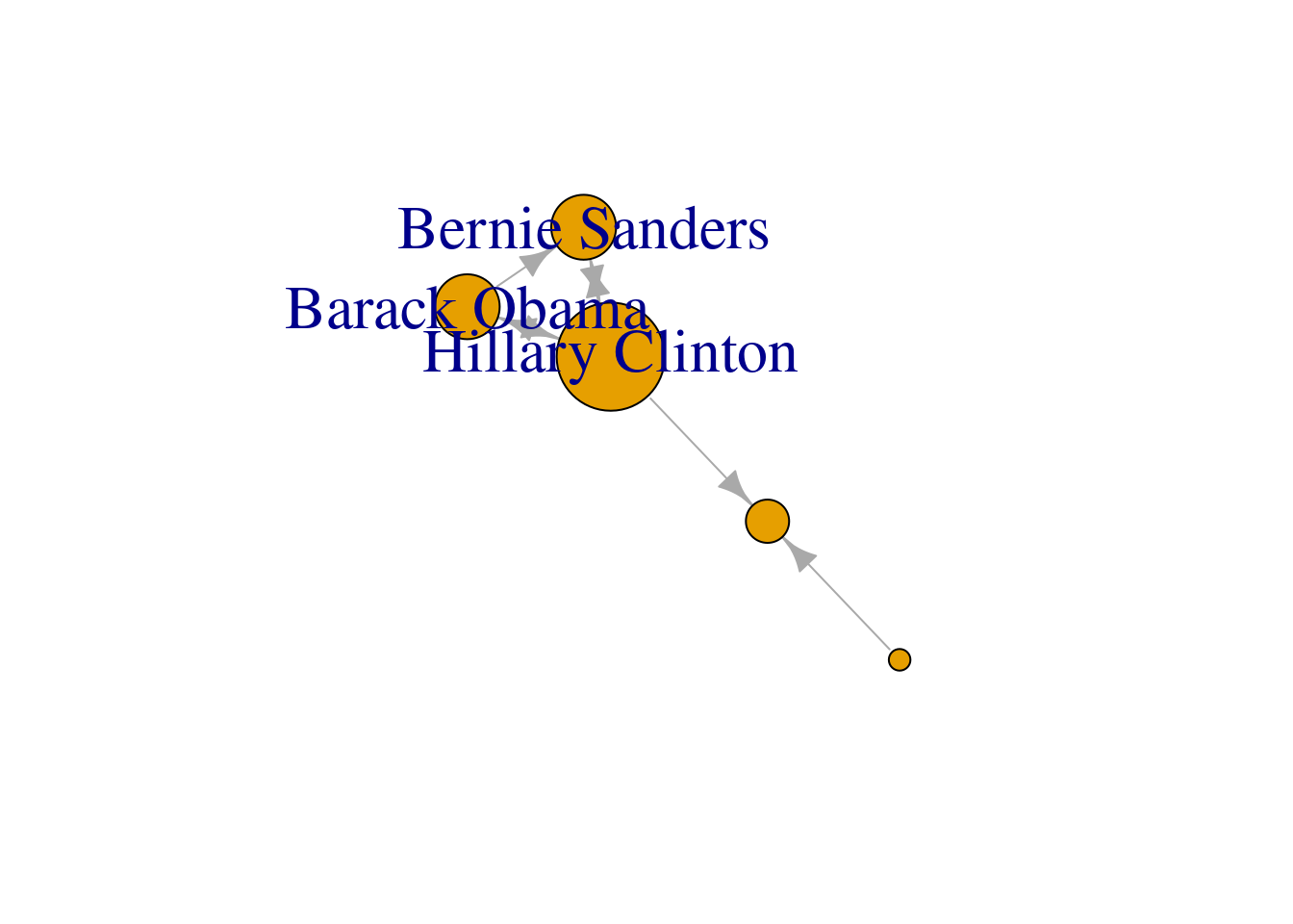
13.2.3 Clustering and Community Detection
One of the greatest potentials of SNA is the ability to identify how nodes are interconnected and thus define communities within a graph. This is to say that most of the time the nodes and edges in our network are not distributed homogeneously, but they tend to form clusters that can later be interpreted. In a social network you can think for example of the principle of homophily, which is the tendency of human beings to associate and interact with similar individuals; or you can think of extrinsic factors (e.g., economic or legal) that may generate the cohesion of small groups of citizens that belong to a wider social structure. While it is of course difficult to make strong claims regarding the underlying causes, we can use different computational approaches to model and detect possible communities that emerge from social networks and even interpret and label those groups. The creation of clusters as an unsupervised machine learning technique was introduced in Section 7.3 for structured data and in Section 11.5 for text analysis (topic modeling). We will use some similar unsupervised approaches for community detection in social networks.
Many social and communication questions may arise when clustering a network. The identification of subgroups can tell us how diverse and fragmented a network is, or how the behavior of a specific community relates to other groups and to the entire graph. Moreover, the concentration of edges in some nodes of the graph would let us know about the social structure of the networks which in turn would mean a better understanding of its inner dynamic. It is true that the computational analyst will need more than the provided algorithms when labeling the groups to understand the communities, which means that you must become familiar with the way the graph has been built and what the nodes, edges or weights represent.
A first step towards an analysis of subgroups within a network is to find the available complete subgraphs in an undirected graph. As we briefly explained at the end of Section 13.1, these independent subgraphs are called cliques and refer to subgroups where every vertex is connected to every other vertex. We can find the maximal cliques (a clique is maximal when it cannot be extended to a bigger clique) in the imaginary undirected graph of American politicians on Facebook (g1) by using the functions max_cliques in igraph (Eppstein, Löffler, and Strash 2010) and max_cliques in networkx (Cazals and Karande 2008). As you can see in Example 13.18, we obtain a total of three subgraphs, one representing the Democrats, another the Republicans, and one more the connector of the two parties (Clinton–Trump).
Now, in order to properly detect communities we will apply some common algorithms to obtain the most likely subgroups in a social network. The first of these models is the so called edge-between or Girvan–Newman algorithm (Newman and Girvan 2004). This algorithm is based on divisive hierarchical clustering (explained in Section 7.3) by breaking down the graph into pieces and iteratively removing edges from the original one. Specifically, the Girvan–Newman approach uses the betweenness centrality measure to remove the most central edge at each iteration. You can easily visualize this splitting process in a dendogram, as we do in Example 13.19, where we estimated cl_girvan to detect possible communities in the Facebook network. We used the functions cluster_edge_betweenness in igraph and girvan_newman in networkx.
Example 13.19 Clustering with Girvan–Newman.
cl_girvan = nxcom.girvan_newman(g1)
# Note: see R output for a nice visualization
cl_girvan = cluster_edge_betweenness(g1)
dendPlot(cl_girvan, mode="hclust")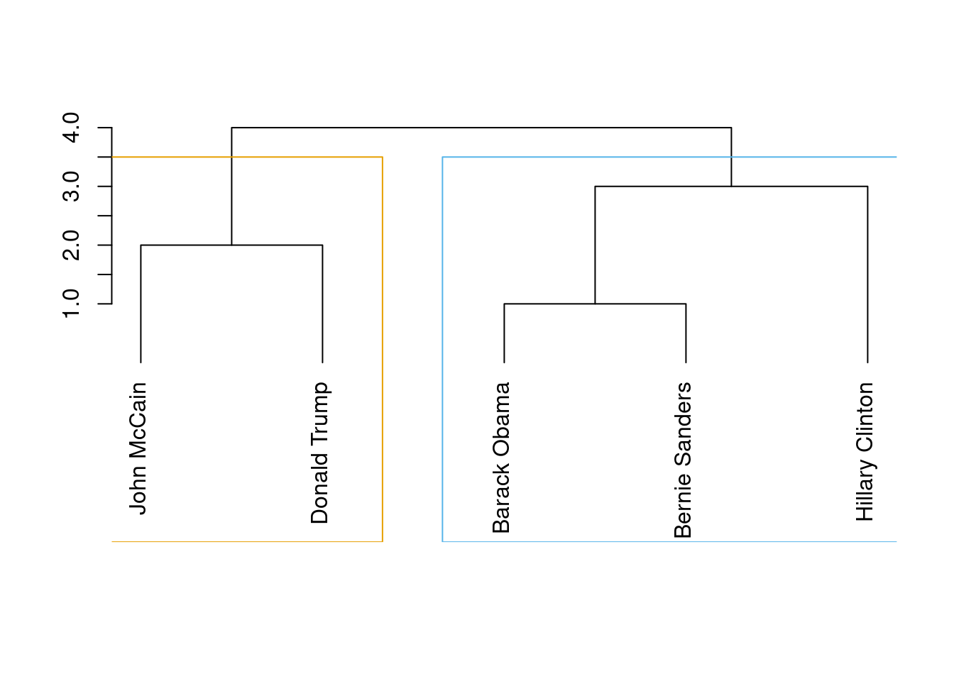
When you look at the figure you will notice that the final leaves correspond to the nodes (the politicians) and then you have different partition levels (1 to 4), which in fact are different cluster possibilities. In edge-betweenness clustering, the big question is which partition level to choose, or in other words, which of the community division is better. The concept of modularity arises as a good measure (\(-1\) to 1) to evaluate how good the division is (technically it’s measured as the fraction of edges that fall within any given groups, let’s say group 1 and group 2, minus the expected number of edges within those groups distributed at random). Thus, we can choose which of the four proposed divisions is the best based on the highest value of their modularities: the higher the modularity the more dense the connections within the community and the more sparse the connections across communities. In the case of cluster_edge_betweenness in igraph it automatically estimates that the best division (on modularity) is the first one with two communities.
With community detection algorithms we can then estimate the length (number of suggested clusters), membership (to which cluster belongs each node) and modularity (how good is the clustering). In the case of igraph in R we apply the functions length (base), membership and modularity over the produced clustering object (i.e., cl_girvan). In the case of networkx in Python we first have to specify that we want to use the first component of the divisions (out of four) using the function next. Then, we can apply the functions len (base) and modularity to get the descriptors, and print the first division (stored as communities1) to obtain the membership.
These functions are demonstrated in Example 13.20. Note that since we will be showing these properties for multiple clustering algorithms below, we create a convenience function summarize_clustering to display them.
We can estimate the communities for our network using many other more clustering algorithms, such as the Louvain algorithm, the Propagating Label algorithm, and Greedy Optimization, among others. Similar to Girvan–Newman, the Louvain algorithm uses the measure of modularity to obtain a multi-level optimization (Blondel et al. 2008) and its goal is to obtain optimized clusters which minimize the number of edges between the communities and maximize the number of edges within the same community. For its part, the Greedy Optimization algorithm is also based on the modularity indicator (Clauset, Newman, and Moore 2004). It does not consider the edges’ weights and works by initially setting each vertex in its own community and then joining two communities to increase modularity until obtaining the maximum modularity. Finally, the Propagating Label algorithm – which takes into account edges’ weights – initializes each node with a unique label and then iteratively each vertex adopts the label of its neighbors until all nodes have the most common label of their neighbors (Raghavan, Albert, and Kumara 2007). The process can be conducted asynchronously (as done in our example), synchronously or semi-synchronously (it might produce different results).
In Example 13.21 we use cluster_louvain, cluster_fast_greedy and cluster_label_prop in igrapgh (R) and best_partition, greedy_modularity_communities and asyn_lpa_communities in networkx (Python). You can see that the results are quite similar6 and it is pretty clear that there are two communities in the Facebook network: Democrats and Republicans!
We can plot each of those clusters for better visualization of the communities. In Example 13.22 we generate the plots with the Greedy Optimization algorithm in R and the Louvain algorithm in Python, and we get two identical results.
Example 13.22 Plotting clusters with Greedy optimization in R and Louvain in Python
# From which cluster does each node originate?
# (note that for Louvain clustering, this actually reverses the preprocessing we did above
#  so we could also have used the original community_louvain(.) output directly.
#  For the networkx community functions this conversion is needed in any case)
clusters = [next(i for (i, members) in enumerate(cl_louvain) if x in members)
            for x in g1.nodes]

pos = nx.spring_layout(g1)
plt.figure(figsize=(6, 3))
plt.axis("off")
nx.draw_networkx_labels(g1, pos, font_size=6)nx.draw_networkx_nodes(g1, pos, cmap=plt.cm.RdYlBu, node_color=clusters)
nx.draw_networkx_edges(g1, pos, alpha=0.3)
plt.show(g1)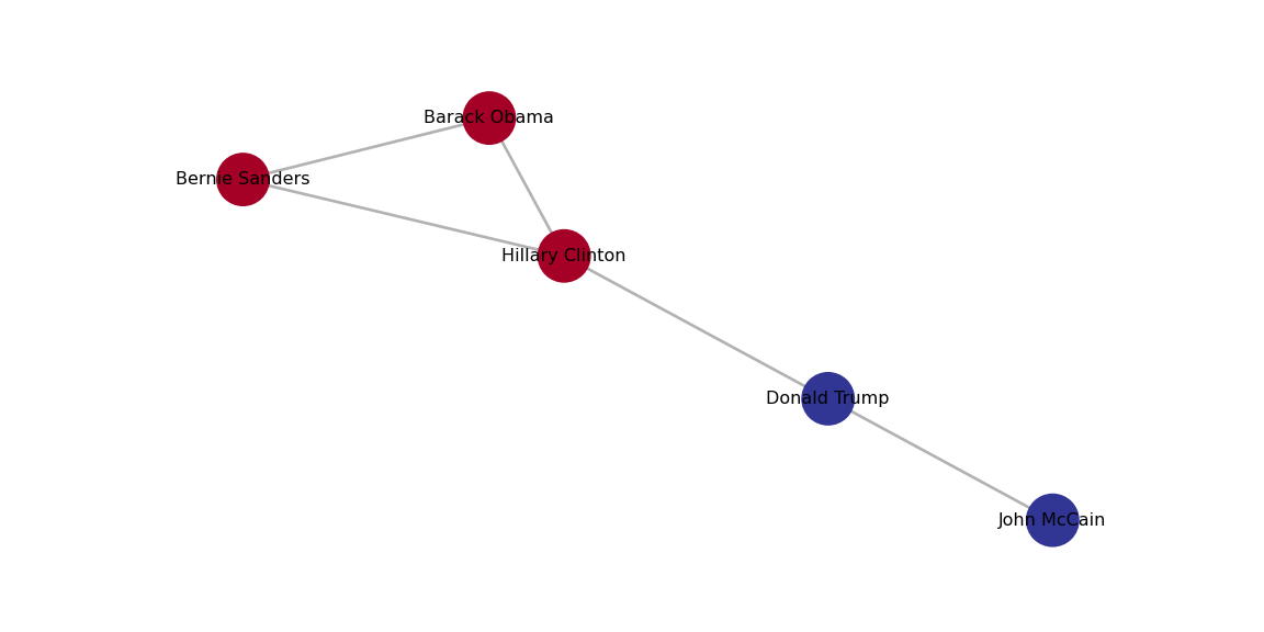
plot(cl_louvain, g1)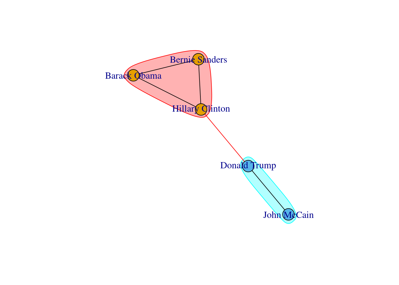
There are more ways to obtain subgraphs of your network (such as the K-core decomposition) or to evaluate the homophily of your graph (using the indicator of assortativity that measures the degree to which the nodes associate to similar vertices). In fact, there are many other measures and techniques you can use to conduct SNA that we have deliberately omitted in this section for reasons of space, but we have covered the most important aspects and procedures you need to know to initiate yourself in the computational analysis of networks.
So far we have seen how to conduct SNA over “artificial” graphs for the sake of simplicity. However, the representation and analysis of “real world” networks will normally be more challenging because of their size or their complexity. To conclude this chapter we will show you how to apply some of the explained concepts to real data.
Using the Twitter API (see Section 12.1), we retrieved the names of the first 100 followers of the five most important politicians in Spain by 2017 (Mariano Rajoy, Pedro Sánchez, Albert Rivera, Alberto Garzón and Pablo Iglesias). With this information we produced an undirected graph7 of the “friends” of these Spanish politicians in order to understand how these leaders where connected through their followers. In Example 13.23 we load the data into a graph object g_friends that contains the 500 edges of the network. As we may imagine the five mentioned politicians were normally the most central nodes, but if we look at the degree, betweenness and closeness centralities we can easily get some of the relevant nodes of the Twitter network: CEARefugio, elenballesteros or Unidadpopular. These accounts deserve special attention since they contribute to the connection of the main leaders of that country. In fact, if we conduct clustering analysis using Louvain algorithm we will find a high modularity (0.77, which indicates that the clusters are well separated) and not surprisingly five clusters.
When we visualize the clusters in the network (Example 13.24) using the degree centrality for the size of the node, we can locate the five politicians in the center of the clusters (depicted with different colors). More interesting, we can see that even when some users follow two of the political leaders, they are just assigned to one of the clusters. This the case of the node joining Garzón and Sánchez who is assigned to the Sánchez’s cluster, or the node joining Garzón and Rajoy who is assigned to Rajoy’s cluster. In the plot you can also see two more interesting facts. First, we can see a triangle that groups Sánchez, Garzón and Iglesias, which are leaders of the left-wing parties in Spain. Second, some pair of politicians (such as Iglesias–Garzón or Sánchez–Rivera) share more friends than the other possible pairs.
Example 13.24 Visualizing the network of Spanish politicians and their followers on Twitter and plotting its clusters
pos = nx.spring_layout(g_friends)
plt.figure(figsize=(10, 10))
plt.axis("off")
size = list(nx.degree_centrality(g_friends).values())
size = [x * 7000 for x in size]
labels_filtered = {
k: v for k, v in nx.degree_centrality(g_friends).items() if v > 0.005
}
labels = {}
for k, v in labels_filtered.items():
labels[k] = k
nx.draw_networkx_labels(g_friends, pos, font_size=10, labels=labels)nx.draw_networkx_nodes(
g_friends,
pos,
node_size=size,
cmap=plt.cm.RdYlBu,
node_color=list(cluster5.values()),
)
nx.draw_networkx_edges(g_friends, pos, alpha=0.5)
plt.show(g_friends)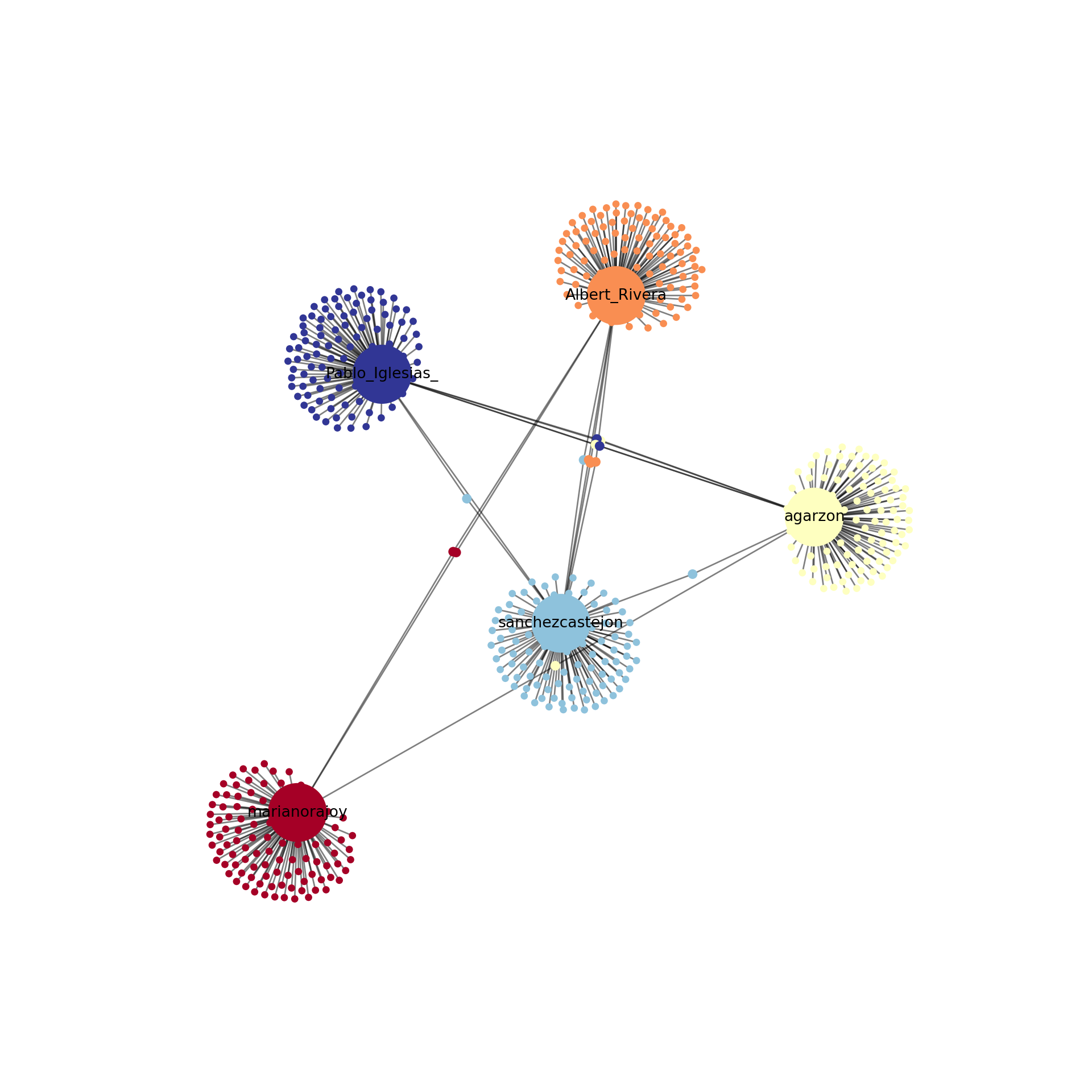
plot(cluster5, g_friends, vertex.label.cex = 2,
   vertex.size=degree(g_friends, normalized=T)*40,
   vertex.label = ifelse(degree(g_friends,
                         normalized=T) > 0.005,
                         V(g_friends)$name, NA))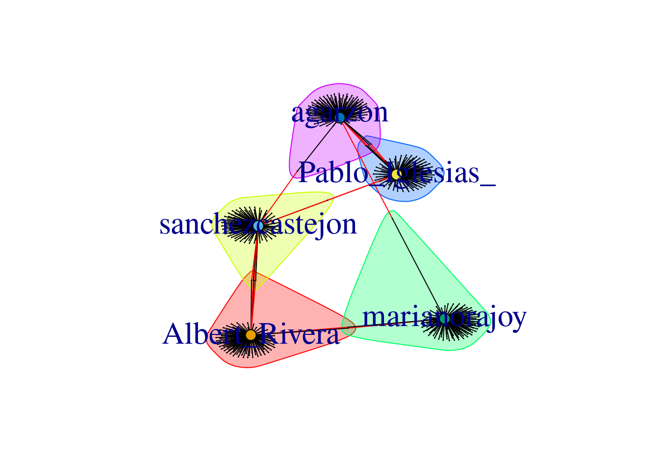
See also the mathematical problem of the Seven Bridges of Königsberg, formulated by Leonhard Euler in 1736, which is considered the basis of graph theory. Inspired by a city divided by a river and connected by several bridges, the problem consisted of walking through the whole city crossing each bridge exactly once.↩︎
The connections among these politicians on Facebook and Twitter in the examples are of course purely fictional and were created ad hoc to illustrate small social networks.↩︎
You can use this library in Python with the adapted package python-igraph.↩︎
The geodesic distance is the shortest number of edges between two vertices↩︎
The approach is to divide by the maximum possible number of vertices (\(N\)) minus 1, or by \(N-1\). We may also estimate the
weighted degreeof a node, which is the same degree but ponderated by the weight of the edges.↩︎This similarity is because our example network is extremely small. In larger networks, the results might not be that similar.↩︎
We deliberately omitted the directions of the edges given their impossible reciprocity.↩︎